
|
The Department of Computer Science & Engineering
|
|
UB CSE 111
|
Searching:
Finding things from a collection of objects occupies a reasonably large amount of our time, and forms the basis of some of our childhood games.
Consider for example the guessing game, where one person mentions they are thinking of a number from, say, 1-100, and will tell you whether their number is higher or lower than any one you guess. This is really just a search problem! Search problems come in other forms too - searching through an unsorted list of names would require looking at every one individually until you find what you're looking for.
Binary Search Trees:
The guessing game can be best solved by first guessing the number middle of the range specified, then continuing to guess in the middle of the new range until the value is found. This is known as binary search. Half of the search space is removed at every step. We can represent this as a tree diagram. Consider the graph for finding items in the range of 1-15:
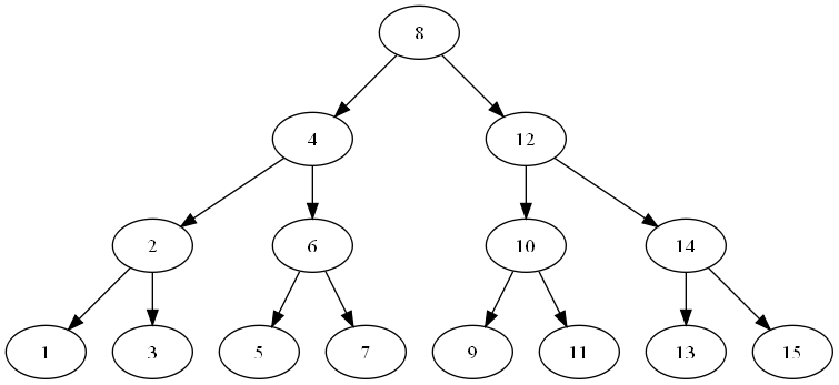
You'll see it will take a maximum of 4 steps to find the solution. Adding another row would allow us another 16 options in the tree, so we would be able to find something in the range of 1-31 in only 5 steps, and so on.
A binary search tree has the property that all items to the left of a node are less than all items to the right. Therefore we know in the graph whether to look left or right if the value we have is less than or greater than the answer. Notice how this only works because the tree gives us a sorting of the data - if it didn't we'd have to look everywhere!
Analysis of Algorithms: Big-O Notation:
It is often useful to analyze the complexity of an algorithm, that is, how 'difficult' an algorithm is to compute. We will be talking mainly about time complexity - that is how long it takes to come to an answer - but there exists other types of complexity like space complexity. We measure the complexity of an algorithm in terms of its input size. We say the size of input is n.
Linear time: O(n)
Assume that you have an alphabetized stack of course registration papers, one for each student at UB. You're looking for some specific student paper and you start at the top of the list looking at each paper until you find what you are looking for. On average you estimate you'll have to look through about half of the stack to find what you are looking for. UB has ~30,000 students, so that's 15,000 papers you'll look through. That's quite a lot to spend the time looking at and inspecting one by one!
We like to generalize our analysis for any length of input though. Therefore we know for a pile of n items, we're going to look through (on average) n/2 items.
Let's look at the graph for y = x and y = x/2.
Notice that the shape of the curve does not change between x and x/2 - only the slope. Therefore both of these functions are called linear and we'll write the complexity of the algorithm as O(n).
Logarithmic time: O(log n)
Consider now that we search the stack of papers using the binary search technique described previously. We first start at the middle of the pile, eliminating either the top or bottom half right away. After one step we have only 15,000 papers to consider. After two, we have 7,500, and after 3 only 3,750. In no more than 15 steps we'll have found the paper we're looking for. This idea of splitting a piece of data in half at every step is the hallmark character of a logarithmic time algorithm. Therefore we say that binary search is O(log n).
(NB: We really mean log2n, which is equivalent to log(n)/log(2), but this is only a linear scaling so we don't worry about writing it down. It's like above - it doesn't change the shape of the graph)
Quadratic time: O(n2)
Consider our naive sorting algorithm. It must look through the entire list of items every time it finds the smallest to add to the new sorted list. That means for n items, it must look through the n item list n times (note this is a rough estimate - the size of the list we're looking through changes, but this estimate is close enough). Therefore we perform n*n steps, and the algorithm is O(n2).
(Note that we include things like n2+n in O(n2) since the lesser term of n doesn't change the shape of the graph here either)
Exponential time: O(2n)
We won't worry about what problems in this class are, but it's worth knowing that they are very very bad. They require performing double the number of operations when the input length increases by only one.
We can look at a graph to see how bad/good each of these are (note x is used instead of n in the graph below):
The table below shows the approximate number of steps needed to complete an algorithm which each complexity for various values of n.
| n = 4 | n = 8 | n = 16 | n = 128 | |
|---|---|---|---|---|
| Logarithmic: O(log n) | 2 | 3 | 4 | 7 |
| Linear: O(n) | 4 | 8 | 16 | 128 |
| Quadratic: O(n2) | 16 | 64 | 256 | 16384 |
| Exponential: O(2n) | 16 | 256 | 65536 | 3.4x1038 |
Notice that as n gets large, the exponential time algorithms get very, very bad. For an input of length 128, 3.4x1038 is A LOT of operations. Let's put that in perspective... A modern 3ghz processor can perform 3 trillion operations per second. Therefore this exponential algorithm would take 113427455640312821154458202477.26 seconds to get an answer. That's about 3596761023602004729656 years. Far, far, far more than the length of the universe!
For more information on Big-O notation, there's a plain-English explanation on the C for Coding blog.
The sorting problem:
We discussed above that searching is much easier if the data we have is sorted... But how do we go about sorting data efficiently? This is a problem many computer scientists have worked on - and for that reason there are a great many algorithms which have been designed for the purpose of sorting data. Many of them are listed on Wikipedia along with the characteristics of the algorithms.
A naive sorting algorithm:
This sorting algorithm looks through an entire list the same number of times as the are numbers of items in the list. This is very similar to the selection sort algorithm (see wikipedia entry), except we have a destination array, while they do it entirely in place by swapping values.
var unsorted[input_count]Let's trace through a sample run. Let's say our value of unsorted is [3, 7, 4].
1. Unsorted is not empty, so we enter our while loop.
2. smallest = MAXVALUE
3. unsorted has items in it, so we set i = 3 and enter the for loop.
4. i is less than smallest (since i = 3 and smallest = MAXVALUE), so we set smallest = 3.
3. We return to step 3 since there are still items we haven't looked at in unsorted. Now i = 7.
4. i (7) is not less than smallest (3).
3. We return to 3 again since there are still items we haven't looked at in unsorted. Now i = 4.
4. i (4) is not less than smallest (3).
5. There are no more items we haven't looked at in unsorted, so we break out of the loop from step 3 and continue on to step 5. We add smallest (3) to sorted. Now sorted = [3].
6. We remove smallest (3) from unsorted. Now unsorted = [7, 4].
Phew, let's take a look at what we've done so far. We've gone through the entire list once looking for the smallest item. We found that it was 3, added it to the beginning of our sorted list, and removed it from our unsorted one. We now return to step 1.
1. Unsorted is not empty, so we enter our while loop.
2. smallest = MAXVALUE
3. unsorted has items in it, so we set i = 7 and enter the for loop.
4. i is less than smallest (since i = 7 and smallest = MAXVALUE), so we set smallest = 7.
3. We return to step 3 since there are still items we haven't looked at in unsorted. Now i = 4.
4. i is less than smallest (since i = 4 and smallest = 7), so we set smallest = 4.
5. There are no more items we haven't looked at in unsorted, so we break out of the loop from step 3 and continue on to step 5. We add smallest (4) to sorted. Now sorted = [3, 4].
6. We remove smallest (4) from unsorted. Now unsorted = [7].
Okay, so now we've gone through our unsorted list again taking out the smallest and putting it at the end of our sorted list. Now lets do this again:
1. Unsorted is not empty, so we enter our while loop.
2. smallest = MAXVALUE
3. unsorted has items in it, so we set i = 7 and enter the for loop.
4. i is less than smallest (since i = 7 and smallest = MAXVALUE), so we set smallest = 7.
5. There are no more items we haven't looked at in unsorted, so we break out of the loop from step 3 and continue on to step 5. We add smallest (7) to sorted. Now sorted = [3, 4, 7].
6. We remove smallest (7) from unsorted. Now unsorted = [].
Now we have to go back to 1 just to make sure that unsorted is empty, and it is, so we now have the sorted array [3, 4, 7].
Analysis:
You'll notice we go through the unsorted list the same number of times as there are items in it for every item it contains. Therefore this algorithm is O(n2).
In lab 2 we split up into groups and each group 'invented' their own sorting algorithm. One sorting algorithm often used both in our everyday lives (without realizing it!) and in computer science is Merge Sort. An intuitive explanation is given below:
We know intuitively that sorting a single number is trivial (clearly it's already sorted!). It's also very easy to keep splitting a list of numbers in half if we know how many we have. Therefore we can see that all the work in the sorting algorithm needs to be done in somehow merging the data back together. We call this general strategy where we split data up into smaller and smaller pieces until it is trivial Divide and Conquer.
The merge step consists of merging two pre-sorted lists (we will start by merging lists of length 1, so we know they are sorted. Then we'll have lists of length 2 which are sorted, and so on). To merge two lists we place a "pointer" at the beginning of both lists. We then choose the lowest value of the two pointers, and move forward whichever pointer whose value we have used. When both pointers are off the end of their respective lists, we are done.
The following animation shows the splitting and merging of a list of numbers to sort it:

The splitting of the initial list is what we call a recursive operation. Recursion is defined as "relating to or involving the repeated application of a rule, definition, or procedure to successive results." We repeatedly apply our "split-in-half" operation to the lists until we have one item (as described above). The below graphic shows how a list is split apart and re-merged.

You should notice that each "row" of merges takes O(n) time (we 'look at' all of the data once every time we do a complete set of merges). You can see the above tree structure shows the number of merge steps to be O(log n). Therefore the algorithm takes O(n log n) time.
An explicit algorithm can be found here, though this is probably too complex for us to think about right now.